
Excel Tips for Data Wrangling: Multiple Criteria Lookups in Excel
This is the second in our ToolTips series on Excel. You can read the first one on V and HLOOKUP here.
Getting Excel to spit out the data you want can be a frustrating exercise sometimes – particularly if there are errors in your formulas! While some of the more advanced lookups can seem overwhelming, breaking them down into their component parts can simplify the process. (This will also help you check for any bugs in your formula that might be causing an error.)
You might be familiar with some of the classic search and lookup functions, such as:
- VLOOKUP—a way to lookup values in a column
- HLOOKUP—a way to lookup values in a row
- XLOOKUP—the modern cousin of the above, allowing vertical and horizontal lookup
- INDEX—a way to return a value in a specific cell
- MATCH—a way to find the location of a value
These are all great functions in their own way, allowing you to find and return specific values you’re looking for in your dataset. But what if you’re searching with multiple criteria?
The classic combination of INDEX and MATCH and the newer XLOOKUP function can both be used to return a value which meets the constraints of a search with multiple criteria.
First, let’s take a look at how an INDEX and MATCH combination can make that happen.
INDEX AND MATCH
The combination of INDEX and MATCH to create an advanced lookup function is popular amongst many Excel users. It involves nesting the MATCH function—used to find the location of a value in a range—inside the INDEX function—used to retrieve the value at a given location. Here’s how it looks:
=INDEX(array, MATCH(lookup_value, lookup_array, match type)
Let’s look at an example. Say we were trying to lookup the February mean maximum temperature for Sydney. In the dataset shown below, we could use the following formula in G3:
e.g. =INDEX(B2:D13, MATCH(G1,A2:A13,0), MATCH(G2, B2:D2, 0))
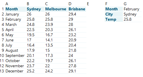
This way, we are dynamically referencing both the row and column lookup; when you change the month (G1) and city (G2), the formula will return the corresponding value from the dataset.
Watch the video below to see how it’s done.
Index and Match with multiple criteria
But what if we had a slightly different problem? What if our dataset was structured differently, and we couldn’t use the MATCH function to return the column index? In this case, we could still use INDEX and MATCH with the addition of multiple search criteria. The generic formula for this looks like the following:
=INDEX(return_range, MATCH(1,(criteria1=criteria_range1) * (criteria2=criteria_range3) * (criteria3=criteria_range3), 0))
If our dataset looked like this:
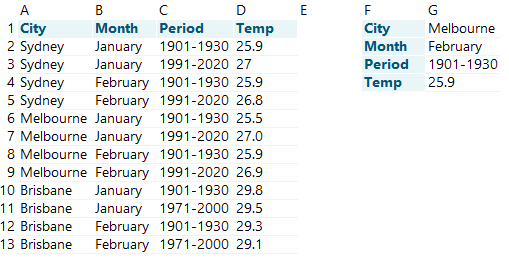
If we wanted to know what Melbourne’s February mean maximum temperature was in the period 1901–1930, we could use the following formula in G4:
e.g. =INDEX(D2:D13, MATCH(1,(G1=A2:A13) * (G2=B2:B13) * (G3=C2:C13), 0))
Watch to see how it’s done.
If you have the most recent version of Microsoft Excel, then this formula will work automatically. If you’re using a slightly older version, you might need to execute it as an array formula using Ctrl+Shift+Enter.
Searching with multiple criteria can also be done using XLOOKUP in a similar way, as shown by the generic formula below:
=XLOOKUP(1,(criteria1=criteria_range1) * (criteria2=criteria_range2) * (criteria3=criteria_range3), return_array)
Hopefully this gives you a bit of an idea of what you can do with the INDEX, MATCH and XLOOKUP functions in Excel.
Enjoy!